Harrison Brammell

Introduction

In this lab, we focused on the use of MATLAB for plotting and function building, specifically exploring key concepts such as writing MATLAB functions, calling those functions, and visualizing data through graphical plots. The lab introduced fundamental MATLAB skills, including creating unit step, ramp, and pulse functions, and emphasized the importance of effective communication of data using visualizations. Through exercises involving function creation and analysis of logical operations, this lab provided a foundation for understanding how MATLAB processes input and output data, as well as how to generate and interpret plots in engineering contexts.

Procedures

Part 1: Matlab Functions

In Matlab, functions are similar to those in other programming languages in that they can be given input and produce an output. They get their own .m file that must live in the directory of the script calling them. For our lab, we implemented the unit step function u(t-to) in Matlab using the code below.

function y = u(t,to)
   %u Unit Step Function
   %y = u(t,to) implements the unit step function, u(t-to).
   %u(t) is 0 for t<to and 1 for t>= to
   y=t>=to;
end

>>t=-5:0.001:5
>>plot(t,u(t,0))

At the end of the code section, you can see the commands we ran in the shell after writing the function. First we declare the domain we want to plot for our function. Then we use the plot command to plot t from earlier versus the unit step function u(t) using our new Matlab function. One thing we experimented with is the step size. Matlab is numerically solving after each step and just connecting the dots, so the more steps we have the more calculations will be made based off of the true unit step function. This means, the smaller the step size the more close the plot will be to the true unit step function.

In MATLAB, the expression “y = t >= to” is a logical operation that compares each element of the array “t” with the value “to”. For each element of “t”, if it is greater than or equal to “to”, the result is 1 (true), otherwise the result is 0 (false). The result is stored in “y” as a binary array, where each position corresponds to whether the condition “t >= to” is met for the respective element in “t”. The array is then treated as a set of points and plotted.

Part 2: Ramp Function

The next function we implemented in Matlab was the ramp, which makes since considering its close relation to the unit step function from part one. The code we used to achieve this can be seen below.

function y = r(t,to)
    % Unit Ramp Function
    %y = r(t,to) implements the unit ramp function r(t - to)
    %returns unit ramp function r = (t,to)
    y = (t-to).*(t>=to);
end

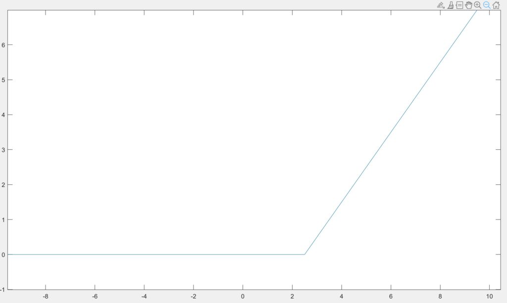
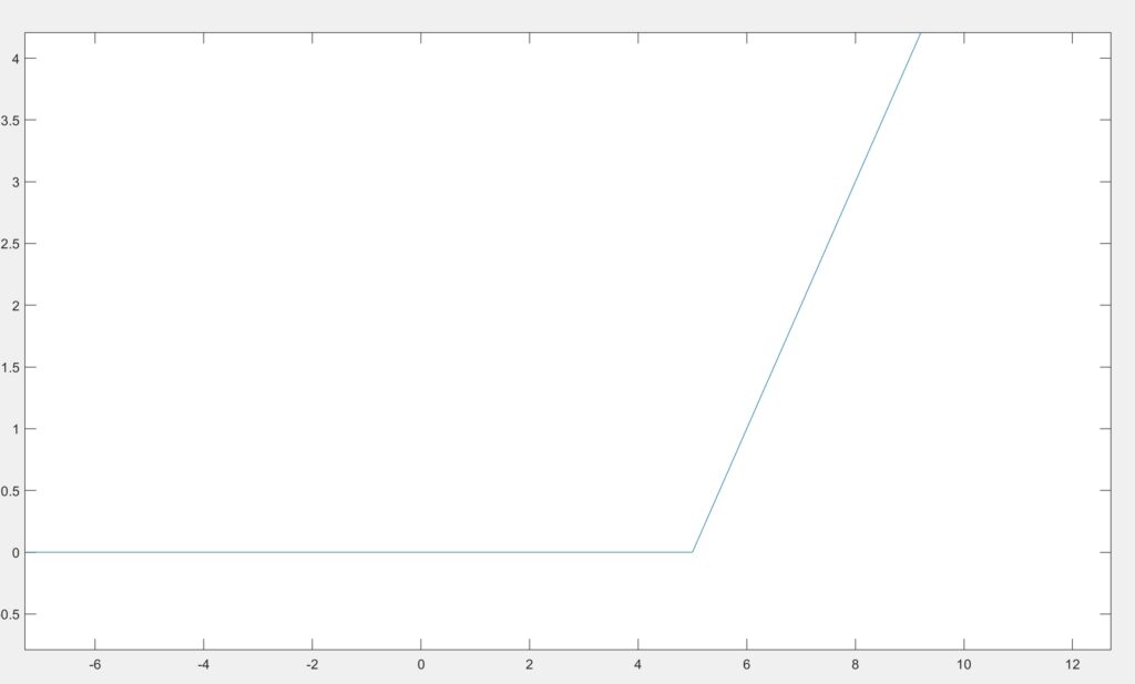
In MATLAB, the expression y = (t – to).*(t >= to) performs two operations. First, it subtracts to from each element in the array t. Then, it uses the logical operation (t >= to) to create a binary array where elements of “t” that are greater than or equal to “to” are marked as 1 (true), and those that are less than “to” are marked as 0 (false). The element-wise multiplication “.*” then multiplies the results of (t – to) by the corresponding binary values from (t >= to), ensuring that for elements of t less than to, the result is zero. This creates a ramp function that starts at to.

We tested the function by plotting two different ramp functions with time delays of 2.5 and 5.0, which can be seen below in figures 2.1 and 2.2.

Part 3: Plotting Skills

For the third exercise, we were set on our own and tasked to recreate two plots. We were told to plot the ramp function r(t) and the unit step function u(t) in the figure but two different plots. We also had to ensure the formatting was correct, including axis labels, adjusting line width, and setting up the domain and range for each of the functions. Below you can find the recreated figures from our Matlab code as well as the code itself.

%Create Array t 
t = -10:0.1:10;

%Create Outputs y = u(t) and y = r(t) 
y_u = u(t,0);
y_r = r(t,0);

%%Step 3
figure(1);
subplot(2,2,1);
plot(t, u(t,0), 'LineWidth',2);
xlabel('Time (s)');
ylabel('Amplitude');
xlim([-10 10]);
ylim([-0.1 1.1]);
title('Plot of u(t)');
grid on;

subplot(2,2,2);
plot(t, r(t,0),'LineWidth',2 );
xlabel('Time (s)');
ylabel('Amplitude');
xlim([-10 10]);
ylim([0 10]);
title('Plot of r(t)');
grid on;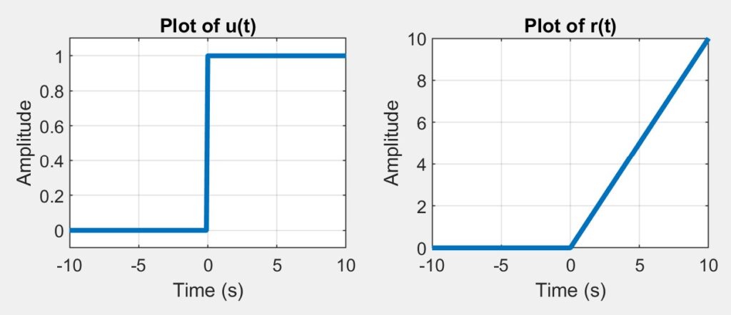

Part 4: Pulse Function

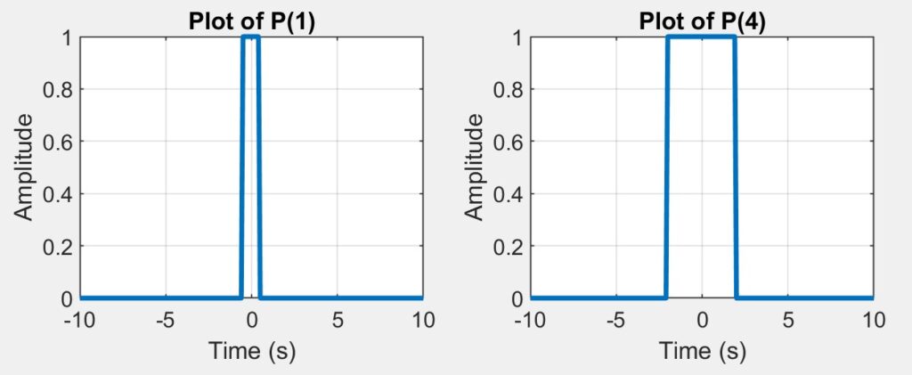
The pulse function is similar to the unit step function. It takes an argument [math]\tau[/math] and gives us a pulse of length [math]\tau[/math]. We implemented this function using the unit step function we implemented earlier. The implementation can be seen below.

function y = pulse(t, tau)
    % Pulse Function
    % y = pulse(t, tau) implements a pulse of width tau centered at t = 0
    y = u(t,-tau/2) - u(t,tau/2);
end

Next, we were tasked with testing our implementation by graphing two plots in a single figure, p(1) and p(4), which can be seen blow in figure 4.1.

Part 5: Building a script with different sections

In MATLAB, sections are blocks of code that can be run independently within a script. Sections are defined by placing %% at the beginning of the line, followed by a space. This visually separates the code into manageable segments, making it easier to organize and debug. Each section can be executed on its own by placing the cursor in the section and clicking “Run Section” in the toolbar, or by using the shortcut key. Sections are especially useful for testing parts of the code incrementally or for organizing complex scripts into logical parts, such as initialization, calculations, and plotting.

The main difference between using subplot and having separate figures in MATLAB is how the plots are displayed. subplot divides a single figure window into a grid, allowing multiple plots to be shown within the same window in different sections, which is useful for comparing plots side by side. On the other hand, using separate figures (figure(1), figure(2), etc.) creates individual, independent figure windows for each plot. This allows each plot to have its own dedicated space, making it easier to view each plot in detail without sharing the same window.

For part 5a, we created a figure containing the plots for all three functions we implemented. We made sure to include these in the same figure and apply the proper formatting functions to meet the requirements of the assignment. The resulting plots can be seen below along with the code used to generate them.

%% Part 5a
figure(3); 
subplot(2,3,1);
plot(t, u(t,0), 'LineWidth',2);
xlabel('Time (s)');
ylabel('Amplitude');
xlim([-10 10]);
ylim([-0.1 1.1]);
title('Plot of u(t)');
grid on;

subplot(2,3,2);
plot(t, r(t,0),'LineWidth',2 );
xlabel('Time (s)');
ylabel('Amplitude');
xlim([-10 10]);
ylim([0 10]);
title('Plot of r(t)');
grid on;

subplot(2,3,3);
plot(t, pulse(t,1), 'LineWidth', 2);
xlim([-10 10]);
ylim([-0.1 1.1]);
grid on;
xlabel('Time (s)');
ylabel('Amplitude');
title('Plot of P1(t)');

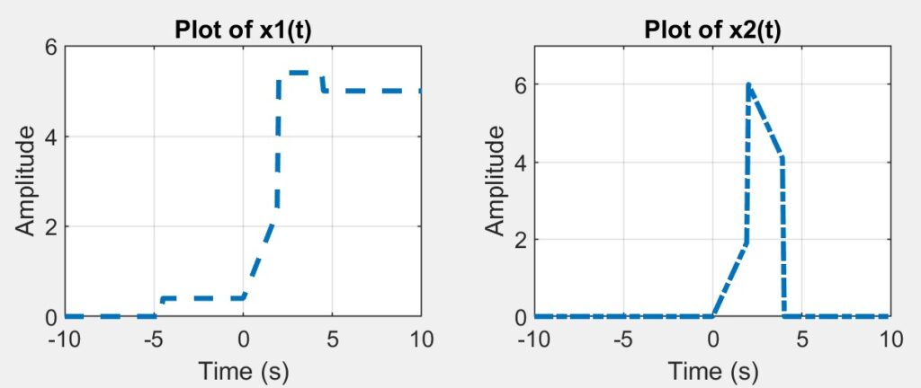
Next for part be, we were assigned the task of generating two plots in the same figure of two functions made up of the transformations and combinations of what we implemented. The functions x1(t) and x2(t) can be seen below in figure 5b.1.

Next, we implemented them using the functions we made. Our approach can be seen below in the code from this section.

%% Part 5b
figure(4);
x1 = (r(t,0)-r(t,2))+(3*u(t,2))+(0.4*pulse(t,9));
subplot(2,2,1);
plot(t, x1,'LineWidth',2,'LineStyle','--');
xlabel('Time (s)');
ylabel('Amplitude');
title('Plot of x1(t)');
xlim([-10 10]);
ylim([0 6]);
grid on;

subplot(2,2,2);
x2 = r(t,0) - 2*r(t,2) + 4*u(t,2) + r(t,4) - 4*u(t,4);
plot(t, x2,'LineWidth',2,'LineStyle','-.');
xlabel('Time (s)');
ylabel('Amplitude');
title('Plot of x2(t)');
xlim([-10 10]);
ylim([0 7]);
grid on;

When this code is run, the following figure is generated. Notice how we changed almost every style aspect of the plots in order to comply with the instructions.

Conclusion

In conclusion, this lab provided a practical exploration of MATLAB’s function-building and plotting capabilities, focusing on creating unit step, ramp, and pulse functions. Through the exercises, we enhanced our understanding of how MATLAB handles logical operations and graphical representations. The lab successfully demonstrated the importance of visualizing data through plots and the efficiency of modular coding in MATLAB. What worked well was the hands-on approach to writing and testing functions, though there were some challenges in getting the plot outputs to match the required format. For future improvements, incorporating more real-time feedback during coding could help smooth the process and enhance understanding.