Harrison Brammell

Introduction

This lab explores the application of Fourier series in digital signal processing using MATLAB. A Fourier series expands a periodic function into an infinite weighted sum of sines and cosines, enabling signal approximation and analysis. However, computational limitations necessitate approximations with finite terms. The lab demonstrates how Fourier series can approximate complex waveforms such as square and triangular waves through MATLAB programming. By incrementally adding harmonics, students will analyze their impact on waveform reconstruction and sound perception. Additionally, the lab investigates the Gibbs phenomenon and computational trade-offs between accuracy and efficiency, providing critical insights into practical implementations of signal approximation.

Procedure

Part A

The code in Part A shows how a Fourier series can approximate a square wave by adding harmonics (odd multiples of the fundamental frequency) using MATLAB. It begins by plotting and playing the sound of the fundamental sine wave, then adds the third harmonic, followed by the fifth, seventh, and ninth harmonics. Each step displays the resulting waveform and plays its corresponding sound. This demonstrates how the waveform changes as harmonics are added and how the plot relates to the sound produced. The code used from the lab manual can be seen below.

%% Plot the fundamental frequency and hear associated sound
t = 0:.1:1000;
y = sin(t);
plot(t,y);
sound(y)
%% Next add the third harmonic to the fundamental, and plot/hear it.
y = sin(t) + sin(3*t)/3;
plot(t,y);
sound(y)
%% Now use the first, third, fifth, seventh, and ninth harmonics.
y = sin(t) + sin(3*t)/3 + sin(5*t)/5 + sin(7*t)/7 + sin(9*t)/9;
plot(t,y);
sound(y)

When we run the code section by section, we can see how as each harmonic is added to the signal it begins to take the shape of a square wave. Additionally, as we listen to each sound produced by the signals applied as an audio output to the speakers of the computer, that each signal changes in tone even though the original tone is still there, just in the presence of another. When we examine the plots, the first is simply a basic sine wave, the second reassembles a sine with some interference, and in the third that interference is exaggerated to point where the signal visually begins to resemble a square wave.

Part B

In part B, we explored the implementation of the Fourier series show in the Matlab code below.

%% CODE 2 - Square Wave
 clc, syms n x
 L = pi; N_TERMS = input('Number of terms: '); n = 1:N_TERMS;
% % Calculating the coefficients of the Fourier Series
% % tic
 a0 = (1/L)*int(1, x, 0, pi);
 an = (1/L)*int(1*cos(n*x), x, 0, pi);
 bn = (1/L)*int(1*sin(n*x), x, 0, pi);
% % Plugging the coefficient values in the Fourier Series
 f = 0;
 for n = 1:N_TERMS
 f = f+ (an(n)*cos(n*x) + bn(n)*sin(n*x));
 end
% % toc
 fprintf('Approximation using %d terms\n', n)
 f_approx = (a0/2)+ f
 ezplot(f_approx, [-10,10])
 title('Fourier Series Approximation')
 xlabel('x')
 ylabel('F(x) approximated')

The code implements the Fourier series by calculating the coefficients a0, an, and bn for the sine and cosine terms using symbolic integration in MATLAB. These coefficients are then used in a loop to build the Fourier series approximation as a sum of sine and cosine functions weighted by the coefficients. The code allows the user to specify the number of terms, which controls the precision of the approximation. Finally, the approximation is plotted to visualize how it compares to the ideal square wave and how it improves with more terms.

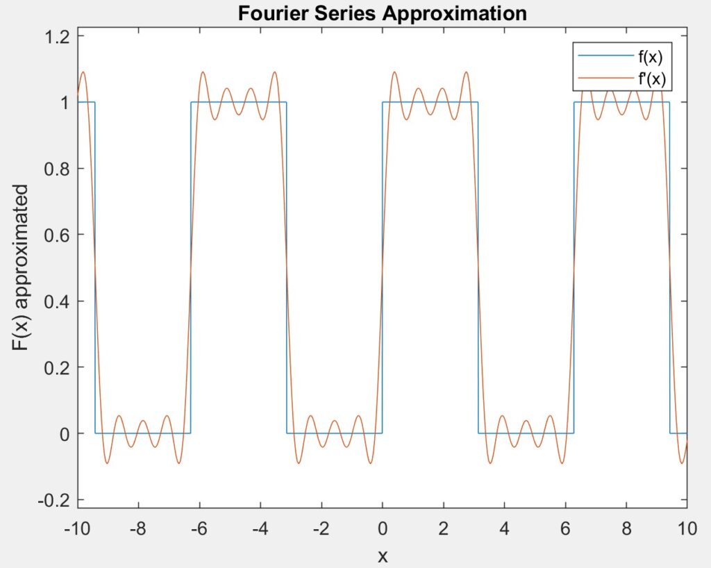
Next, we plotted the ideal square wave on the same graph as a Fourier approximation with seven terms in the summations in order to compare the as shown in the figure below.

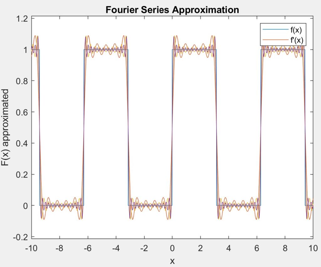
Next, we reran the code multiple times without closing the figure in order overlay multiple different approximations over each other. Below, you can see the graph of the ideal square wave overlayed with approximations of 10, 20, and 30 iterations.

When we examine the graphs, we notice that in some places such as when the ideal square wave is rising or falling, the approximations seems to be very close to the true values, On the other hand, there is a much more noticeable difference at the edges where the function has to make a sharp or where the derivative is a non-zero value.

To further investigate this overshoot, we measured it at increasing number of terms for the approximation as shown in the table below.

Approximation	Overshoot due to Gibbs Phenomenon
7	0.09211
10	0.09014
20	0.08949
30	0.08477
50	0.08466

When we examine the data, we see that even as the numbers of terms in the approximation starts to grow rapidly, the variation in the overshoot gets smaller and it approaches a value around 0.0846, almost resembling exponential decay with an asymptote at that value. This is because of what is called the Gibbs Phenomenon, which describes how Fourier approximations briefly overshoots the true value of the function it approaches at discontinuities at such values. Additionally, no matter how many terms are used this value always settles around 9% of the true value which explains that asymptotic behavior we found in our data.

Next, we examined how the number of terms in the approximation affects the computational time. To do this, we used the tic and toc commands to record the computational time for numerous different values of n and record the data in the table below.

Number of Terms	Computational Time
7	0.082078
10	0.098608
20	0.159070
30	0.230872
50	0.345917
100	0.665613

When we examine this data, we see that while the accuracy of the approximation grows with the number of the number of terms it also makes it computationally more complex and requires more and more time. This poses the question of when the accuracy becomes no longer worth the increased time needed to compute. In order to choose a good number of terms, we must optimize this trade off. While this must be considered on a case-by-case basis, a good rule of thumb could be to choose the first number where the approximation no longer changes within the window of precision necessary for the that specific use case. This both avoids errors and saves us from unnecessary computation time.

Part C

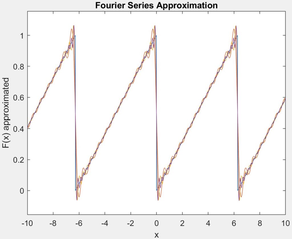
For this part, we performed the same exploration as in the previous section however we focused on the sawtooth wave. In order to do this, we first wrote a section that plots the ideal sawtooth wave, then we used that section to translate the code from the square wave. Finally, we ran the code for 10, 20, and 30 iterations of the approximation and overlayed the resulting graphs with the ideal signal. The results can be seen in the figure below.

Conclusion

In conclusion, this lab provided a hands-on exploration of the Fourier series and its application in approximating periodic waveforms using MATLAB. Through the implementation and analysis of various harmonics, the lab demonstrated how the accuracy of the approximation improves with the inclusion of more terms while highlighting the computational trade-offs involved. The investigation into the Gibbs phenomenon revealed the limitations of the Fourier series near discontinuities, emphasizing the practical challenges of waveform reconstruction. Overall, this lab reinforced the importance of balancing precision and efficiency in signal processing and deepened understanding of how mathematical concepts translate into computational tools for real-world applications.