Harrison Brammell

Introduction

In this lab, we will explore how to solve an AC circuit using Laplace transforms and MATLAB. The circuit under analysis is based on the EQ system from a Fender Blues Jr. Guitar Amplifier, which controls the bass, middle, and treble values—similar to the controls found on a car radio. By transforming the circuit into the Laplace domain, we will utilize mesh analysis to calculate the impulse response when the input is set to a delta function. Through MATLAB, we will verify our results and further analyze the circuit’s behavior. This hands-on exercise will help deepen our understanding of circuit analysis using computational tools.

Procedure

Section 1

Section 1.1: Transform the circuit into the Laplace domain

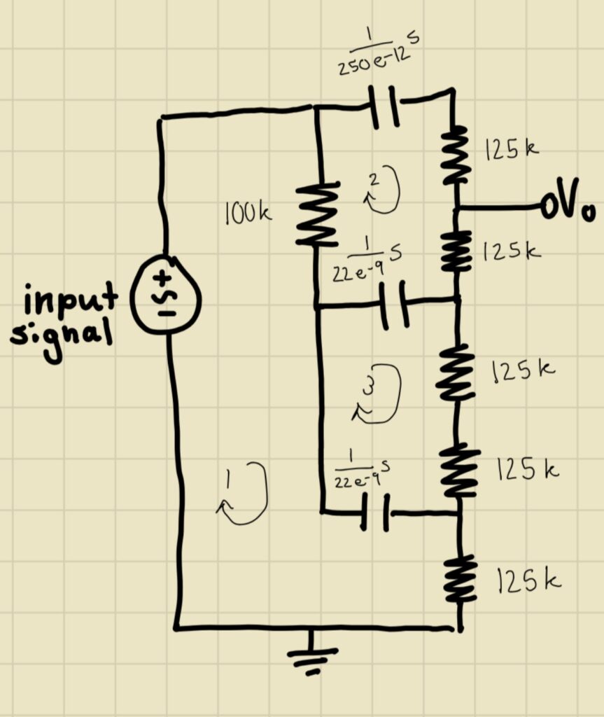
For this part of the lab, we began by transforming our circuit diagram to the Laplace domain. This one done using the equations we learned in electric circuit analysis that state resistor have the same value in the S domain, capacitors take a value of S times the inverse of their value in the time domain, and inductors have a value equal to S times their time domain value. This can be seen in the diagram below.

Section 1.2: Impedance Matrix

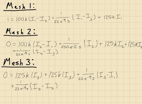
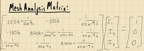
For the next step, we were tasked with finding the impedance matrix for the circuit based off of the diagram we created in section 1.1. This is essentially done by simply performing mesh analysis, and the resulting impedance matrix can be seen below along with the equations used to find the matrix.

Section 2

In this section, we derived an equation for output voltage of the amplifier. V_out was derived by applying KVL to the given circuit in order to create this equation for the output node of the circuit. We apply KVL to find the voltage of its neighboring nodes which we then can compare to find the voltage of V_out as a function of the resistor and capacitor value variables we defined in the beginning of the lab. Essentially, KVL was used starting at the output and finishing at the ground node.

Next, we created two variables, N and D, to represent the simplified numerator and denominator of the output given when we use the simplify function on V_out. All the code and results for these calculations can be seen in the MATLAB code attached to the end of the report.

Section 5

In Section 5, we normalized the polynomial coefficients of the numerator (Np) and denominator (Dp) derived from the Laplace-transformed circuit’s output voltage expression. First, we calculated Np and Dp using the sym2poly() function to convert the symbolic expressions into polynomial arrays. Then, to simplify the values, we divided both Np and Dp by the largest coefficient among them. This normalization step helps in reducing large values and prepares the coefficients for more manageable calculations in subsequent analysis. We also investigated why Np(1) appeared as zero after normalization.

After some tinkering and consultation with the documentation, the reason as to why Np(1) returns zeros becomes clear. While it could be the result of a rounding error, it is likely due to an interesting dynamic with the normalization factor.

If the maximum value k (from [Np, Dp]) is significantly larger than the elements in Np, dividing by k could lead to very small values in Np, which might round to zero due to limited numerical precision.

Section 6

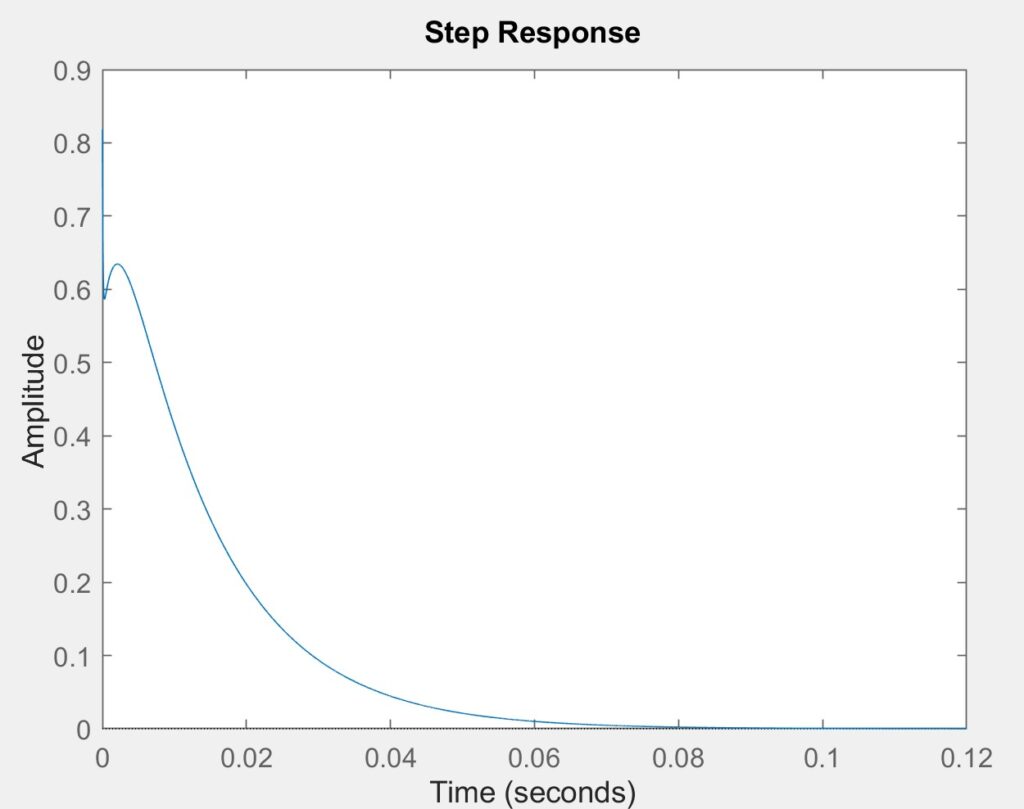
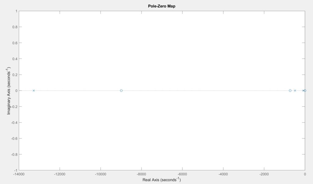
In Section 6, we created a transfer function HHH using the normalized polynomial coefficients Np and Dp, which represent the numerator and denominator of the system’s transfer function. Using the tf() command from MATLAB’s Control Systems Toolbox, we defined H and then analyzed it by plotting key characteristics. We generated a bode plot, a step response, and a pole-zero map to understand the system’s frequency response, transient behavior, and stability. These visualizations provide insight into how the system responds to various inputs and how its poles and zeros influence the overall dynamics and they can be seen below.

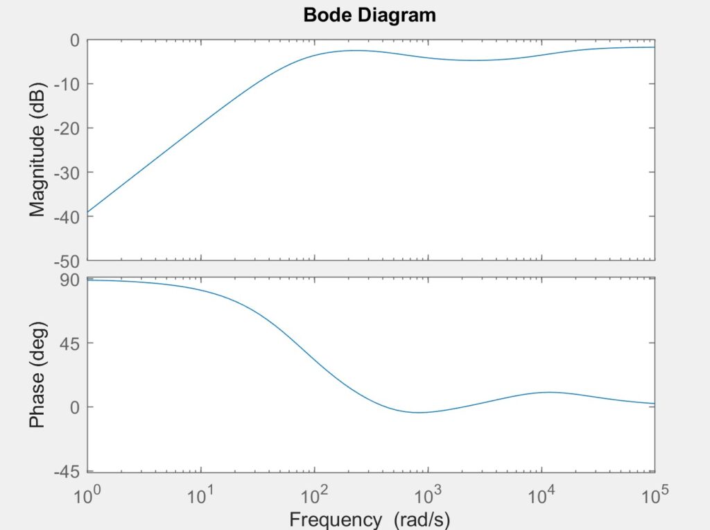
We were then tasked with providing a guess as to what exactly the bode plot represents with respect to the system as a whole. When we look into what exactly this plot could be describing, we come to the conclusion that it is most likely a representation of how the transfer function acts at different frequencies of input signal. This would make sense because the x-axis of these two plots is s or the frequency input into the transfer function which is inheritably in the s domain or the frequency. Additionally, this would make sense considering the Bode has two graphs in it too represent the two components of the transfer functions phasor.

When considering the shape, we see that between 10^2 and 10^3 rad/s that the frequency response of the system (made up of both components graphed in a bode plot) begins to stabilize where as before it clearly was exhibiting some change. This could indicate that around that frequency range the systems becomes stable and the effect of frequency on the systems output begins to have little to no effect.

Conclusion

In conclusion, this lab provided valuable insight into analyzing electrical circuits using Laplace transforms and MATLAB tools. Through each section, we applied mesh analysis, derived output voltage equations, and explored symbolic simplifications to create a transfer function that models the circuit’s behavior. One of the challenging aspects was ensuring accuracy in MATLAB, where a small error in defining the transfer function—mistakenly using tf(Np, Np) instead of tf(Np,Dp) which led to incorrect results. Debugging this highlighted the importance of precision in coding for accurate system analysis.

Overall, it was rewarding to see how these tools are applied in a way that mirrors professional engineering practices. Analyzing the system as a whole, rather than simply solving isolated equations, provided a more holistic understanding of how engineers approach and model complex systems in real-world applications. This experience deepened my appreciation for MATLAB’s capabilities in professional circuit analysis.