Introduction
In this lab report, we explore the poles and zeros of continuous transfer functions, using MATLAB to analyze and manipulate system dynamics. A transfer function, expressed as the ratio of a system’s output to its input in the Laplace domain, provides critical insights into system behavior. By identifying poles (values where the transfer function approaches infinity) and zeros (values where the transfer function becomes zero), we can determine a system’s stability, classify its response characteristics, and visualize behavior through tools such as impulse response and pole-zero maps. This lab emphasizes practical applications, guiding the construction of transfer functions, stability analysis, and pole-zero cancelation techniques to stabilize or optimize system performance.
Exercises
Part 1
For the first part of the lab, we were tasked with analyzing the system defined by the differential equation seen in the figure below. Additionally the transfer function generated from the Matlab code provided to us can be seen below as well.


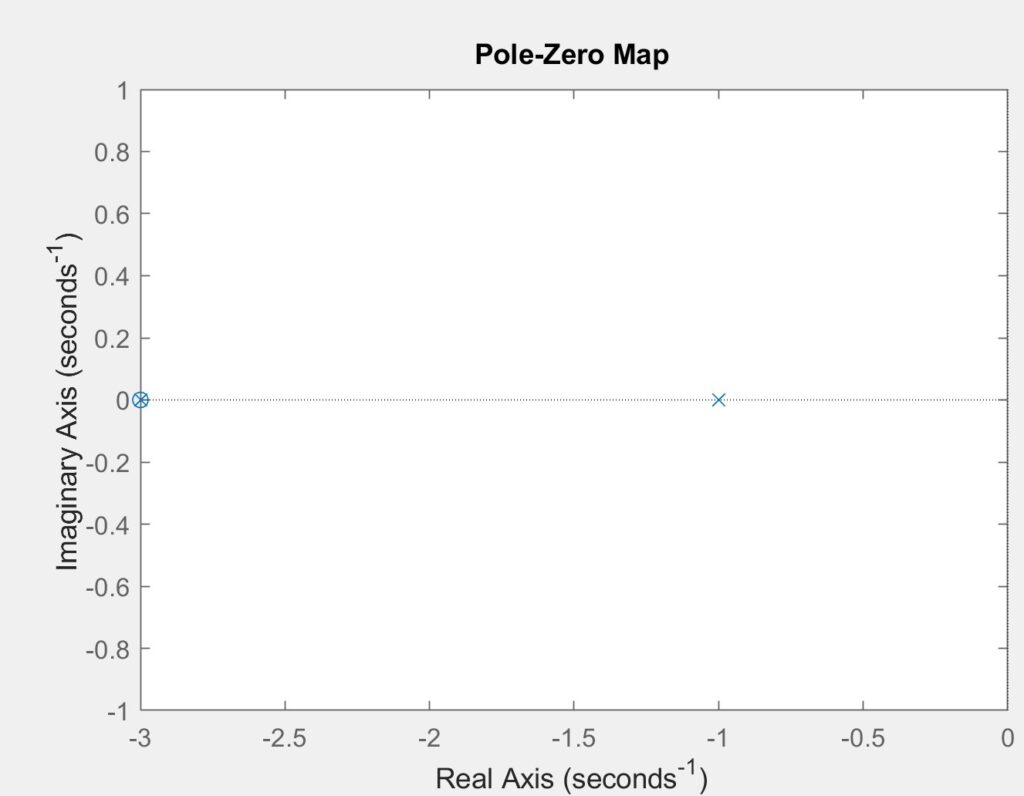
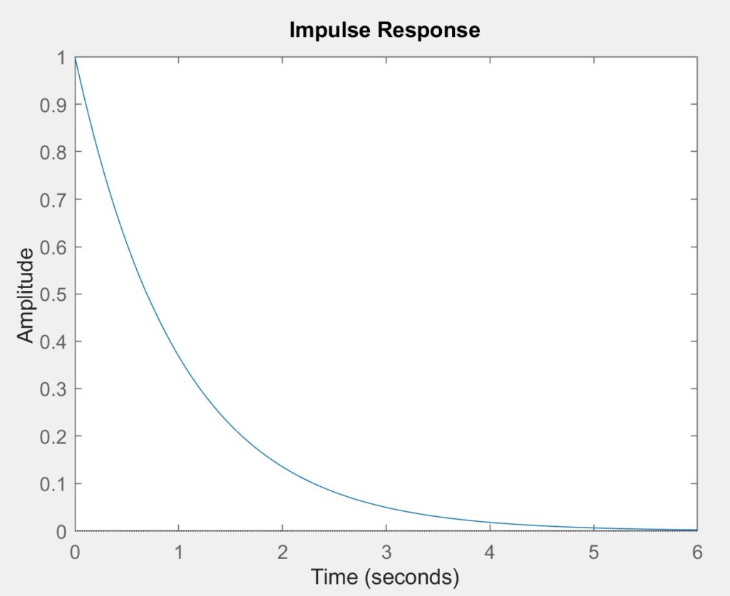
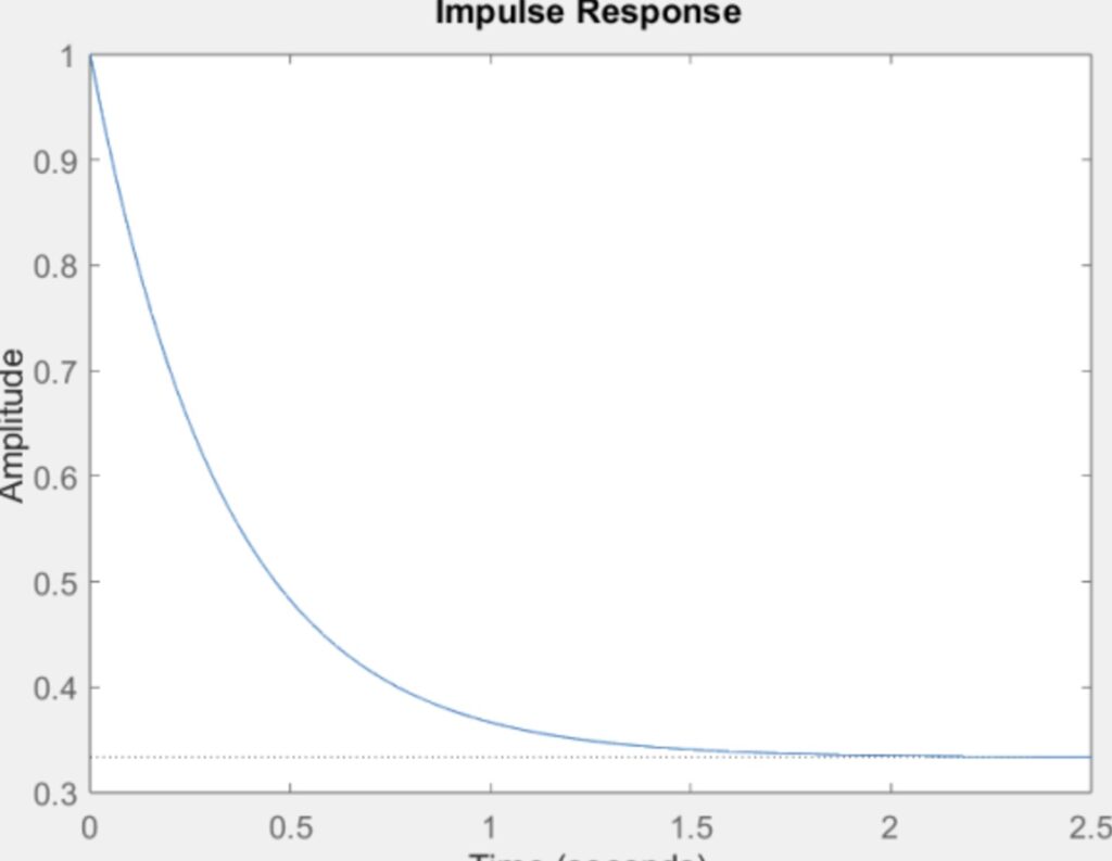
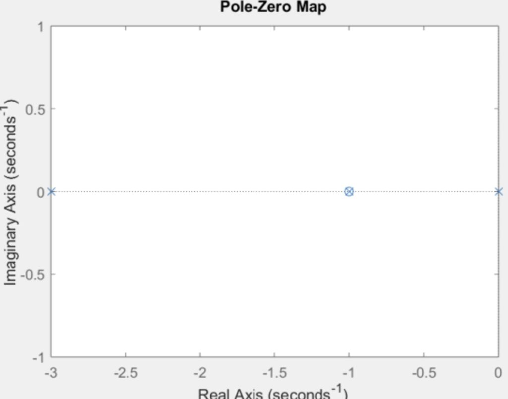
When we look at the pole-zero map, we can see that the system has a zero at z=-3, and two poles at -1 and -3 and this can be seen in the figure below. The system is asymptotically stable as it approaches zero over time. Stability is ensured because all poles have negative real parts, which also confirms asymptotic stability. This behavior is evident in the impulse response, which decays to zero over time.
Part 2
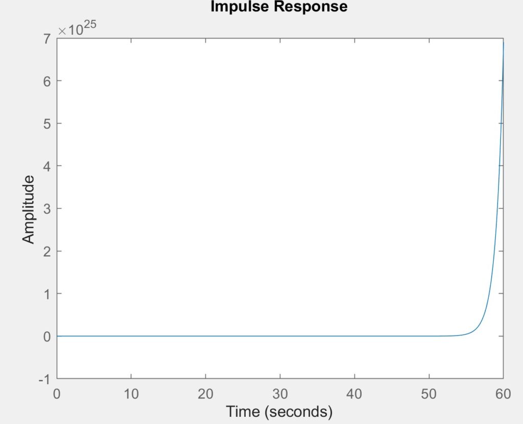
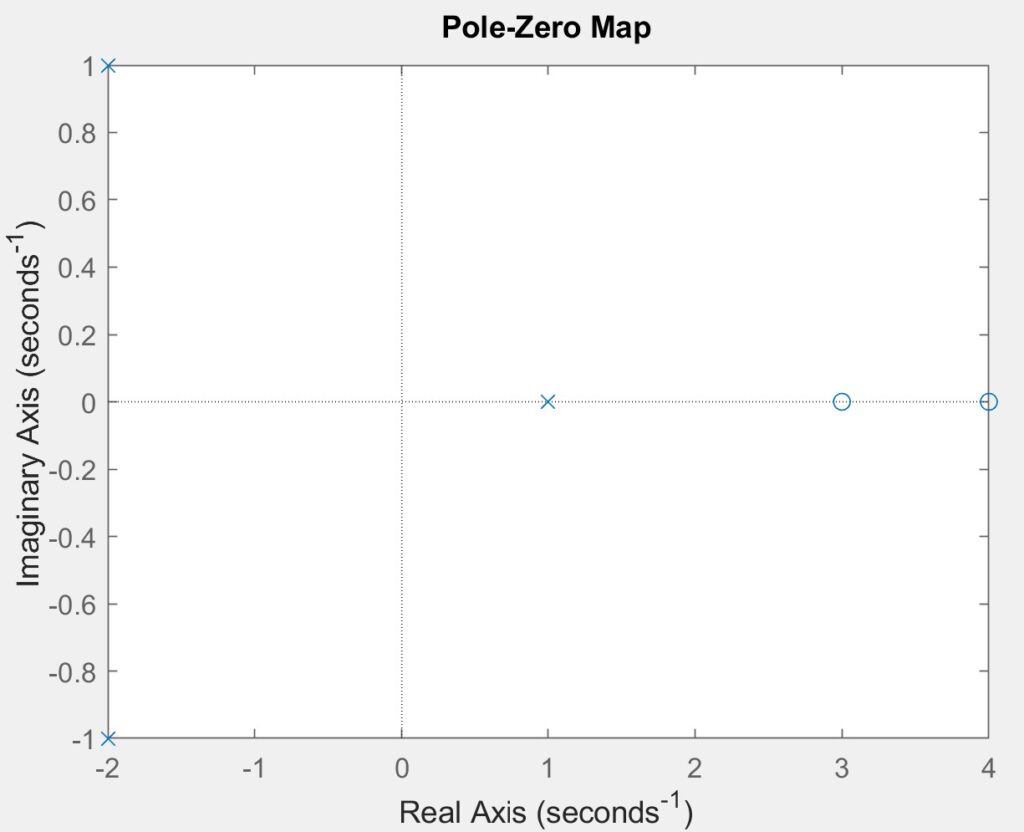
The poles are p = -2 + j, -2 – j, 1 + j0 and zeros of this equation are z = 3, 4. The system is unstable as it grows without bounds. This instability arises because at least one pole has a positive real part. As shown in the figures, the impulse response increases indefinitely.


Part 3
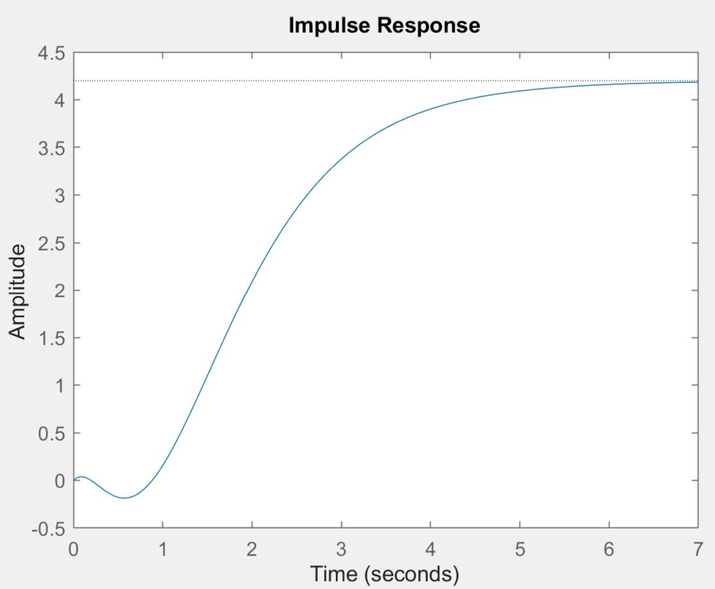
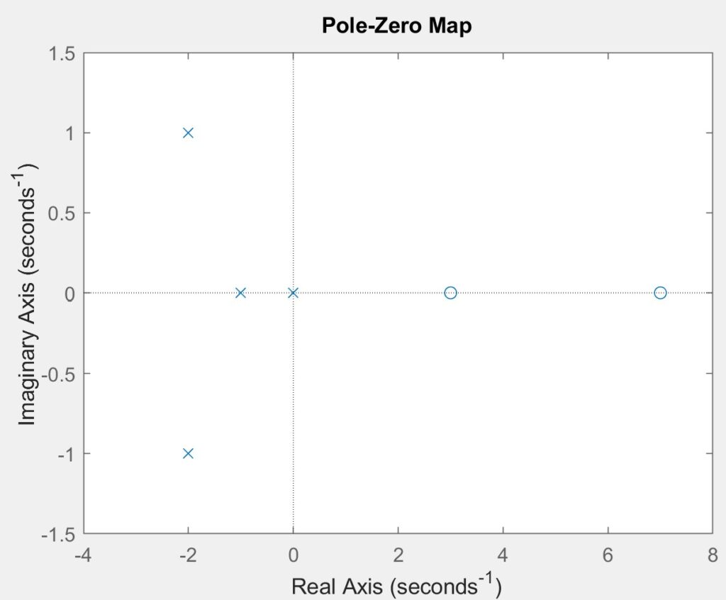
The poles of this equation are 0, -1, -2 + j, and -2 – j, while the zeros are 7 and 3. The system is stable as it remains bounded by a constant. However, it is not asymptotically stable due to the presence of a pole at zero. The figures demonstrates that the impulse response is confined within a constant value.


Part 4
With the help of some online tutorials I was able to design the function below to meet the specifications given in the lab manual. The system is stable because all poles are less than or equal to zero. However, it is not asymptotically stable due to the presence of a pole at zero.

Part 5
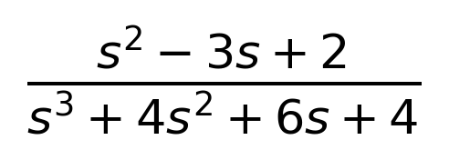
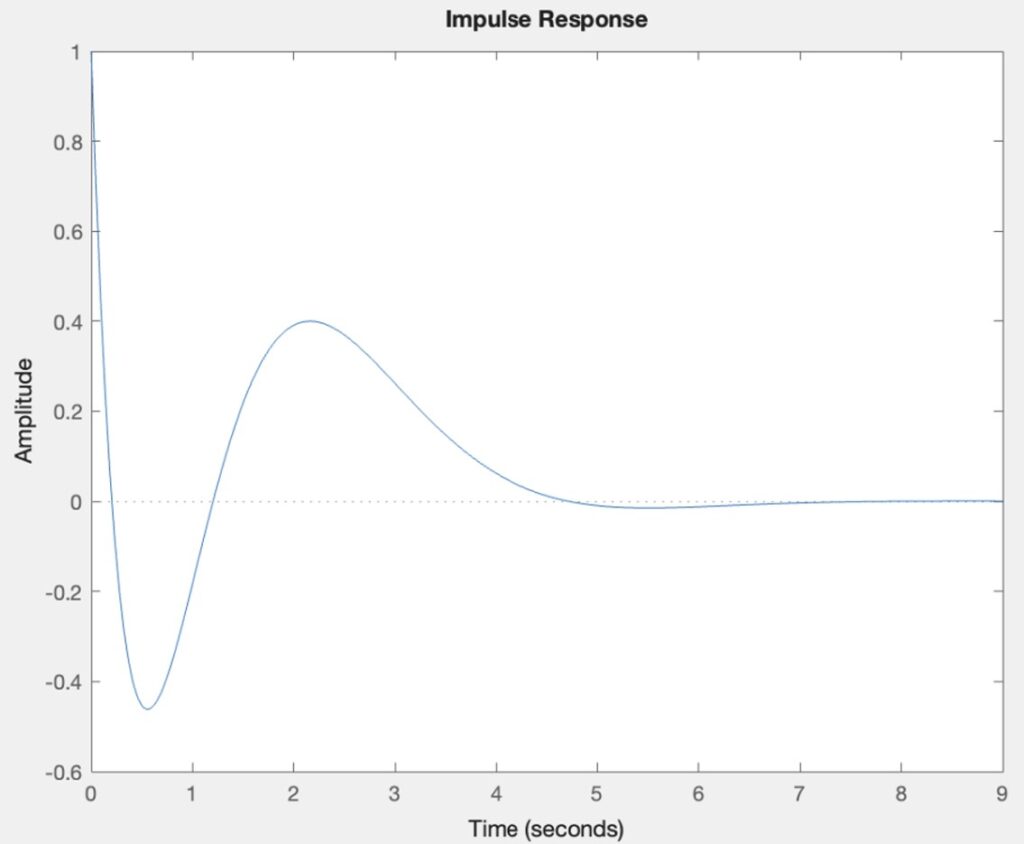
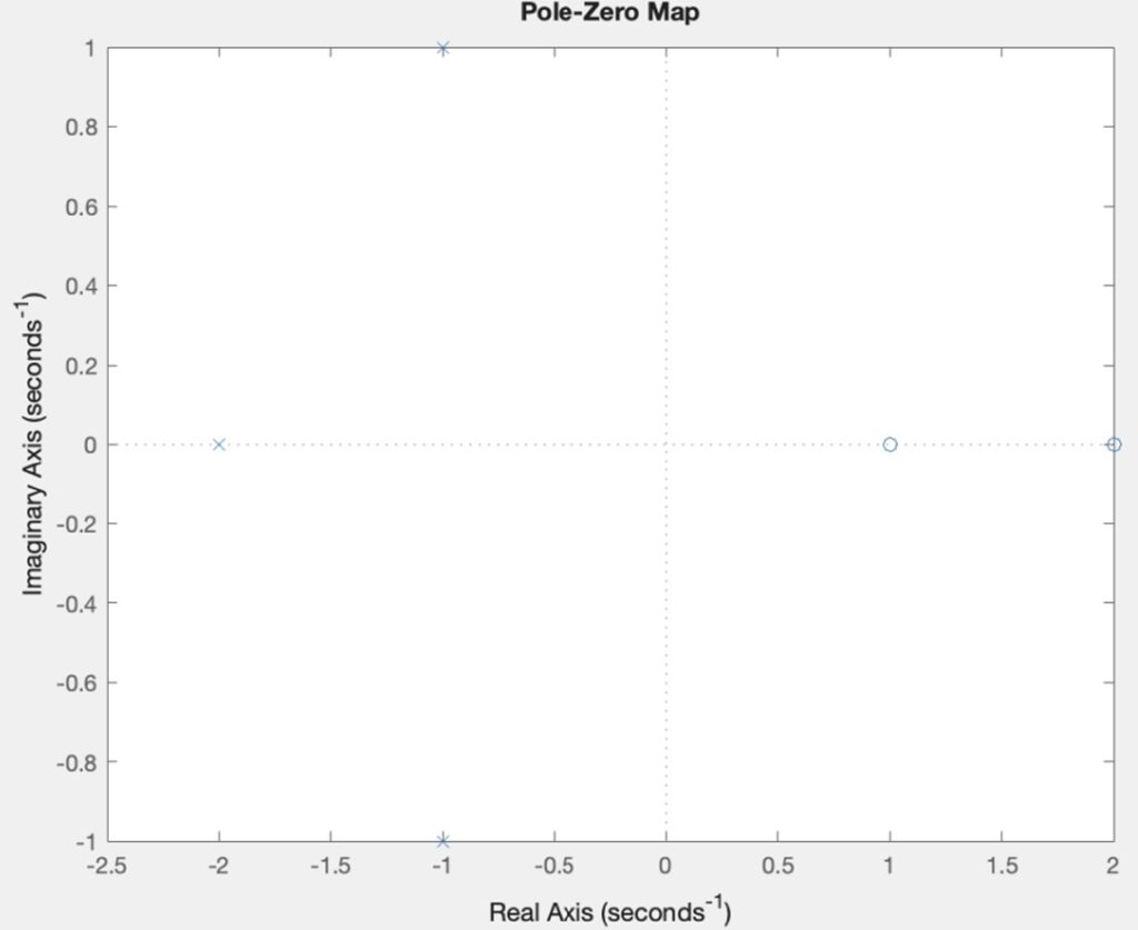
The system is asymptotically stable because its impulse response approaches zero as time progresses. This stability is further confirmed as the real parts of all poles are strictly negative.
Part 6
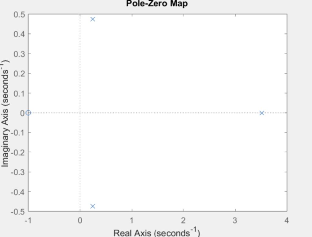
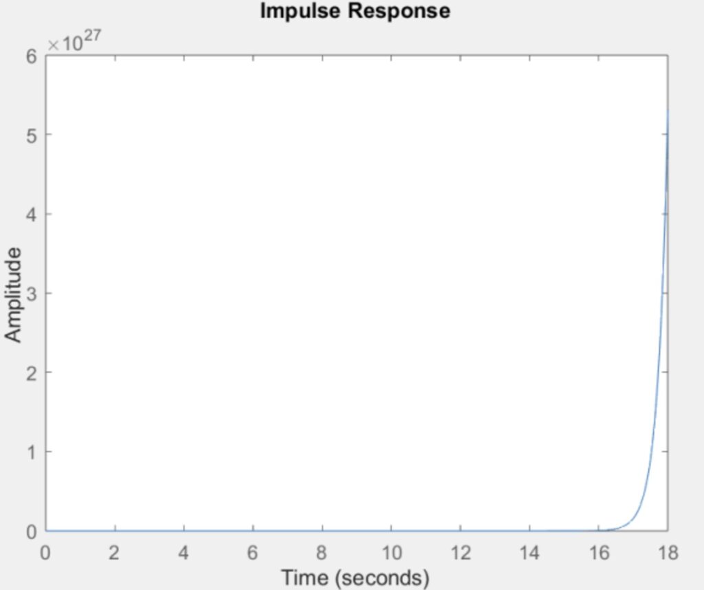
This system is unstable because there are poles that are greater than 0.

Part 7
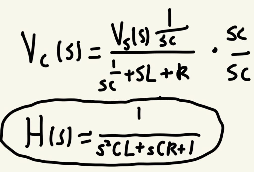
The transfer function can be seen below.
Part 8
Part 9
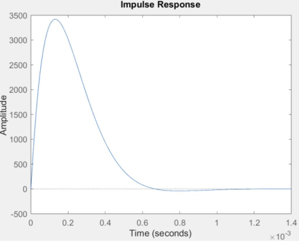
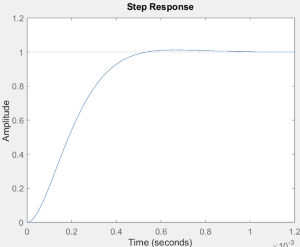
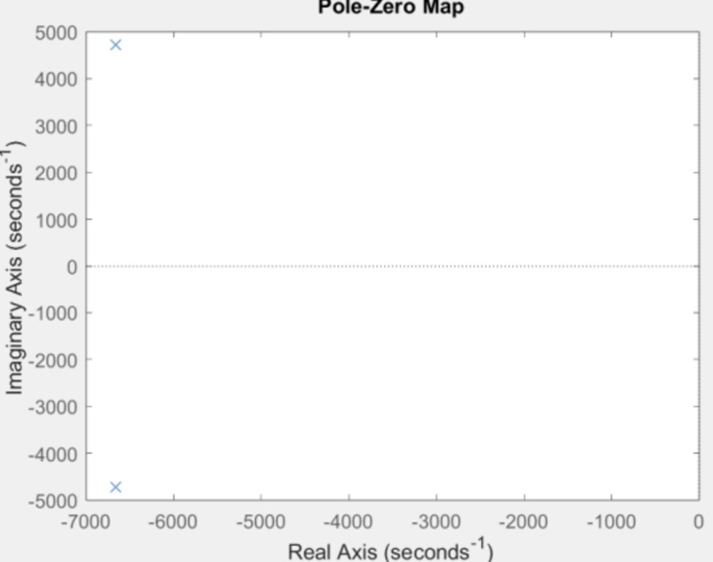
The poles are -6670 + 4710i and -6670 – 4710i, and there are no zeros. The system is asymptotically stable because it converges to zero, as the real parts of the poles are negative.
Part 10
The system is asymptotically stable because it approaches zero, given that the real parts of the poles are negative.
Part 11
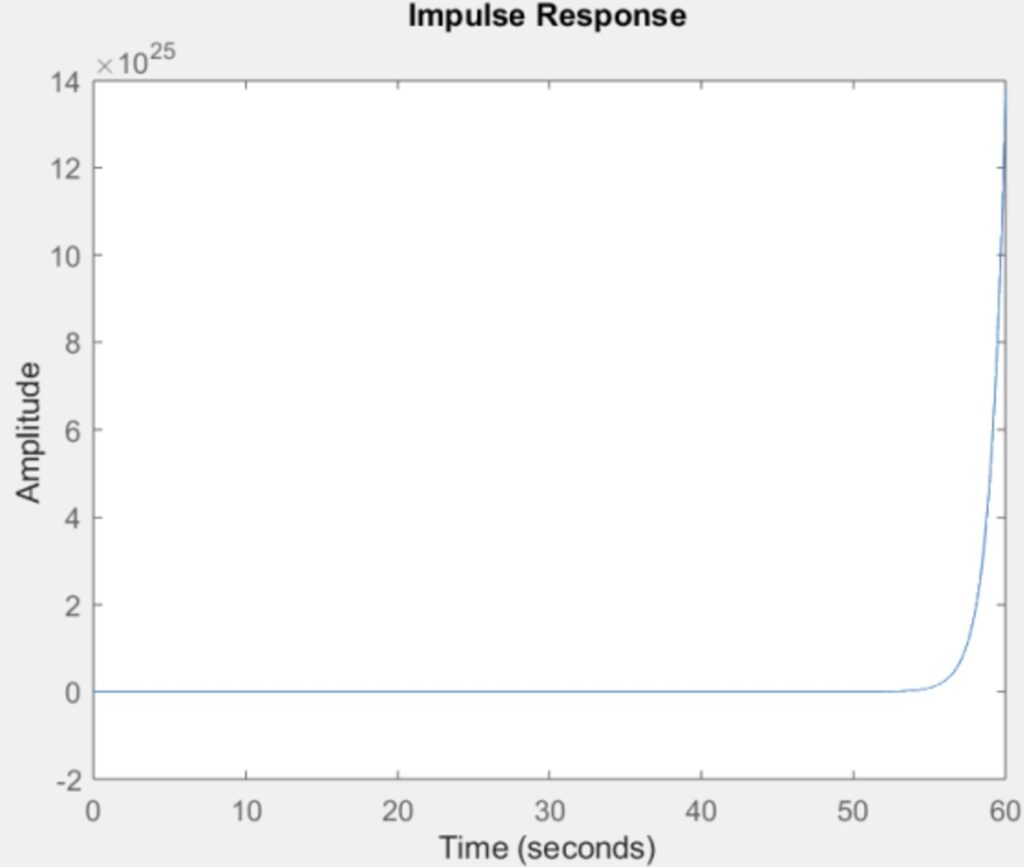
We can immediately see the function is unstable because it is trending towards infinity. The function is unstable because the poles are 1, -1 + j, and -1 – j, and the zeros are 3 and 4. The instability is caused by the pole at 1, which is greater than zero.

Part 12

Part 13
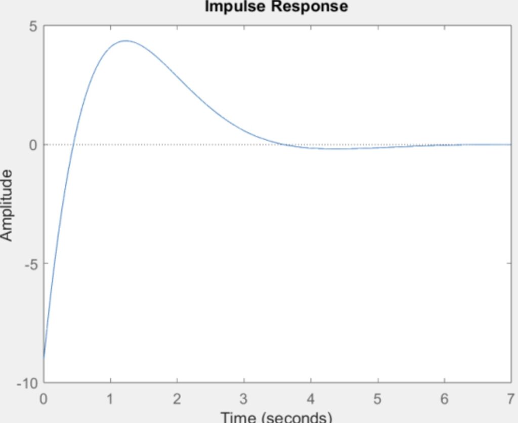
The system is now asymptotically stable because all the real parts of the poles are negative. This outcome was expected since the unstable pole was removed.


Conclution
This lab provided a comprehensive understanding of the poles and zeros of continuous transfer functions and their critical role in system analysis and stability determination. Using MATLAB, the lab demonstrated methods to compute poles and zeros, visualize their locations using pole-zero maps, and assess system stability through impulse and step responses. Key insights included the distinction between stable, unstable, and asymptotically stable systems and the significance of pole-zero cancellation in stabilizing unstable systems. The exercises reinforced theoretical concepts by integrating practical computation and analysis, offering a solid foundation for further exploration in control systems and dynamic modeling.
Leave a Reply